Introduction
In this lab, I iteratively designed a turbine to extract power from wind tunnel flow (20 m/s), attempting to maximize extracted power. I used QBlade for blade optimization and design (the program includes a basic BEM environment) and PTC Creo to construct the turbines. The turbines were then 3-D printed from ABS. Our designs were, of course, subject to constraints: a maximum diameter of 0.15 m and print time of 8 hours. The scientific concepts of this lab were essentially equivalent to those of the last lab; attempting to optimize the coefficient of power, \(C_P\), required a thorough understanding of lift (which I tried to increase) and drag (which we attempted to decrease). Lift on a global scale is the result of a transfer of momentum from a fluid to a wing, and on a local scale the result of pressure forces on the wing. By the simplified "equal paths" explanation, air must travel farther, and thus, faster over the top of an airfoil than the bottom, causing a net difference in pressure above and below the wing, observed as lift. Unfortunately, even flat plates can create a great deal of lift, and that paths should be traveled in equal time is far from obvious. Einstein, subscribing to this theory of lift, attempted to design his own airfoil. After a biplane fitted with the foil flew like a “pregnant duck,” Einstein commented, “[this] is what can happen to a man who thinks a lot but reads little,” (Seelig 251). Jamieson provides a more nuanced explanation. Flowlines following the curved upper profile of an airfoil are directed down, a vertical change in momentum. Flowlines follow the profile because of the pressure field the airfoil generates: in accelerating the flow around the profile, local pressure is reduced, causing the flow to “stick” to the surface. To create a well-performing airfoil is to create a shape that maximizes the curve, change in direction of flowlines, for a specific flow without separation. Drag can be understood in terms of momentum or energy. When an object passes through a fluid, it necessarily changes not only the momentum of the fluid in the direction perpendicular to its motion (lift) but also parallel to that motion (drag). Conservation of momentum or kinetic energy indicates that this increase in momentum or kinetic energy of the fluid is associated with a decrease in the momentum or kinetic energy of the object: drag. Design was complicated somewhat because the motion of the blades of our turbine was radial, not linear; effective velocity scaled linearly along the length of a blade as did the effects of our design parameters. Our intuition was therefore of more limited use. We, nevertheless, completed three prototypes, experiencing for the first time in this course iterative design (actual engineering).
Definition of Problem and Parameters
We are instructed to design a wind turbine that extracts the maximum of power from the flow. Flow is steady (20 m/s) and near uniform, though, as it is contained in a duct 0.61 m x 0.91 m, some velocity gradients are present. Turbine diameter must not exceed 0.15 m, no flow directing devices are permitted (duct), and the turbine must operate about an axis aligned with the flow (HAWT). Our designs are to be 3-D printed, and print time must not exceed eight hours. Performance under different loads is determined from voltage and frequency measurements of a brushless generator (motor) coupled to our turbines. Load is varied by changing the resistance of the circuit.
Design
I attempt a rigorous optimization procedure. The design parameters that result in maximal power production (measured by \(C_P\), coefficient of power) have been largely derived for turbines under the provided (rather textbook) conditions: fixed pitch, fixed freestream velocity, and specified radius.
We begin with the equation for optimal (\(C_P\)) non dimensional lift distribution for such a scenario, as derived in most BEM texts. We use Jamieson's notation and equation numbering. Making the usual BEM assumptions, independence of performance across annular rings (flow across interior airfoils does not influence those further out), no wake expansion, and steady flow, we have (1.50)
\[\frac{c(\lambda,x)C_L}{R} \equiv \Lambda(\lambda,x) = \left(\frac{8\pi a (1-a)}{B\lambda(1+a')\sqrt{(1-a)^2+\lambda^2x^2(1+a')^2}}\right)\left(\frac{F}{1+\frac{(1-a)}{k \lambda x (1+a')}}\right)\] and
\[a' = \frac{\sqrt{\lambda^2k^2x^2+2\lambda k x-4a k [\lambda x-k(1-a)] +1 } - (\lambda k x + 1)}{2\lambda k x} \longrightarrow^{k\to\infty} \frac{\sqrt{4a-4a^2+\lambda^2x^2}-\lambda x}{2\lambda x}\] \[\approx \frac{a(1-a)}{\lambda^2 x^2}\] in which \(x = \frac{r}{R}\) is the normalized distance from the origin (axis of rotation), \(\lambda\) the tip speed ratio, \(C_L\) the local coefficient of lift, \(a\) the axial induction factor, \(a'\) the tangential induction factor, \(B\) the number of blades, \(F\) a correction for tip losses, and \(k\equiv\frac{C_L}{C_D}\) the ratio of the lift and drag coefficients.
Tip speed ratio \(\lambda\) is the ratio of the blade tip's tangential velocity to the freestream velocity \(V_\infty\)
\[\lambda\equiv\ \frac{V_{tip}}{V_\infty} = \frac{\omega R}{V_\infty}\] in which \(\omega\) is the angular frequency of the blade and \(R\) its radius.
The axial induction factor \(a\) is the fractional reduction in freestream velocity local to the rotor (1.2);
\[W_{ext} = U_\infty(1-a)\] in which \(W_{ext}\) is the local velocity.
The tangential induction factor \(a'\) is the mean fractional increase in tangential velocity local to the rotor (tangential velocity is zero in freestream flow but is imparted by the turbine, rising across a blade to \(2a'\omega\) directly downstream);
\[W_{tang} = \omega r(1+a') = \lambda x(1+r')\]
We use the Prandtl tip factor to correct for tip losses. \[F = \frac{2}{\pi} \arccos\left[\frac{-B\lambda(1-x)}{2(1-a)}\right]\]
For optimal \(C_P\), the derivation of the Betz limit specifies \(a = \frac{1}{3}\). Our twist distribution is then given by (1.73)
\[\theta(\lambda,x) = \arctan\left[\frac{2}{3\lambda x(1+a')}\right]-\alpha_0(x)\] in which \(\alpha_0(x)\) is the angle of incidence at which the airfoil section achieves maximal \(k\). Jamieson proceeds to assume that \(a'\) is small, a valid approximation, he asserts, so long as \(\lambda > 6\), in which case
\[\Lambda(\lambda,x) \approx \frac{16\pi}{9B\lambda^2x} \longrightarrow c(\lambda,r) \approx \frac{16\pi R^2}{9B C_L \lambda^2 r}\] and
\[\theta(x) = \frac{2}{3\lambda x}-\alpha_0(x)\] pleasant simplifications valid for large turbines. Unfortunately, our \(\lambda < 6\).
We must now choose an airfoil. We calculate the Reynolds number for a blade (2.4):
\[R_e = \frac{W c(\lambda,r)}{\nu_{air}} \approx \frac{\omega r c(\lambda,r)}{\nu_{air}} = \frac{16 \pi R U_\infty}{9 B C_L \lambda \nu_{air}} = \frac{16 \pi (0.15 m)(20 m/s)}{9 (B) C_L (1) (1.568*10^{-5}) } \] Our \(R_e \approx 15000\) for \(B\) between 4 and 10 and \(C_L\) between 30 and 40. This sweeping \(R_e\) approximation is valid as most of the power is produced in the midsection of the blade. Obviously, local \(R_e\) varies widely. We begin with a simple, single-airfoil design. We select the SG6043 (at maximum \(\frac{C_L}{C_D}=39.7\), \(C_L \approx 1.4\)) with the aid of New Airfoils for Small Horizontal Axis Wind Turbines's useful figure (Figure 2) as it is optimized for small wind turbine design (if much larger \(R_e\)).
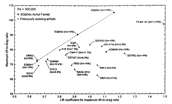
Its performance figures over a range of \(R_e\) are provided from XFoil simulations on AirfoilTools and are shown in Figure 3.
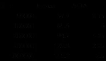
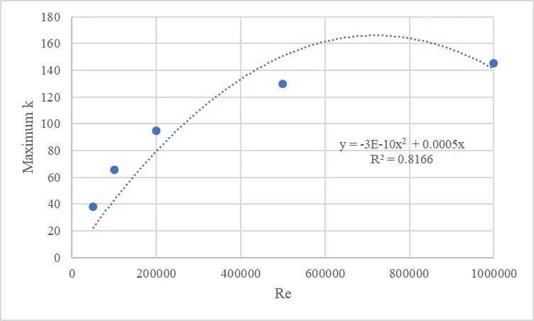
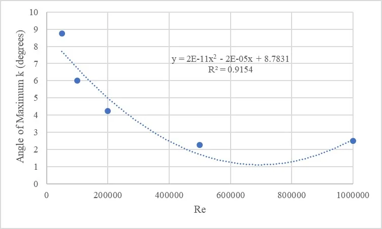
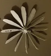
To maximize \(C_P\) in this \(R_e\) regime (see Figure 1.10), we wish to maximize \(B\) (Jamieson 257). Increasing the maximum \(C_L\) of the airfoil decreases optimal chord \(c(\lambda,r)\); to maximize \(B\) we wish to minimize the chord of each blade (to material limits). As our first trials demonstrated, the resolution of the printer must also be kept in mind; if inaccurately rendered, all of our optimization is worthless. In practice, the twelve blades of Design I held up well, but the tips were poorly formed by the printer. The blade profile as a function of the number of blades can be viewed in the attached Mathematica notebook. We decide (rather arbitrarily) to use twelve blades, presuming that a larger number would be rendered defectively. We compute the expected \(k\) and \(\alpha_0\) for the airfoil at \(R_e \approx 15 000\). Fitting the provided data for large \(R_e\) to quadratic order (Figure 4), we calculate \(k \approx 7.5\)(!) and \(\alpha_0 \approx 9.1\). While \(\alpha_0\) has not shifted much, \(k\) is clearly highly dependent on \(R_e\). As such, I linearize it, assuming that our calculated \(R_e\) holds for \(x = 1/2\). That is, \(k = 2*7.5x\).
We now calculate \(c(\lambda,r)\) (Figure 5(a)) and \(\theta(\lambda,r)\) (Figure 5(b)) for twelve blades.
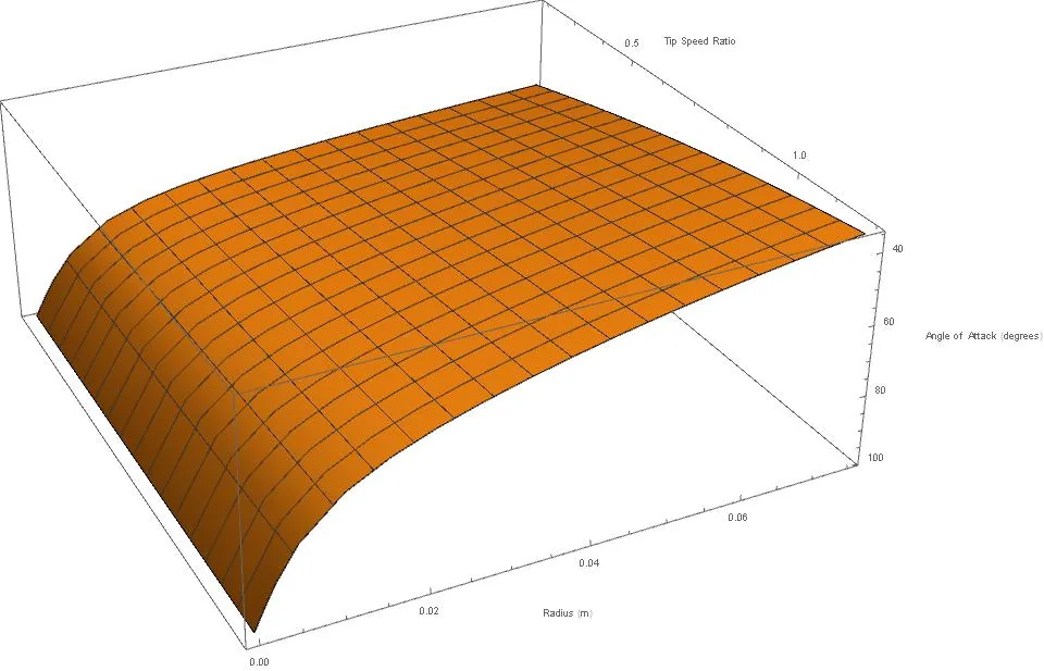
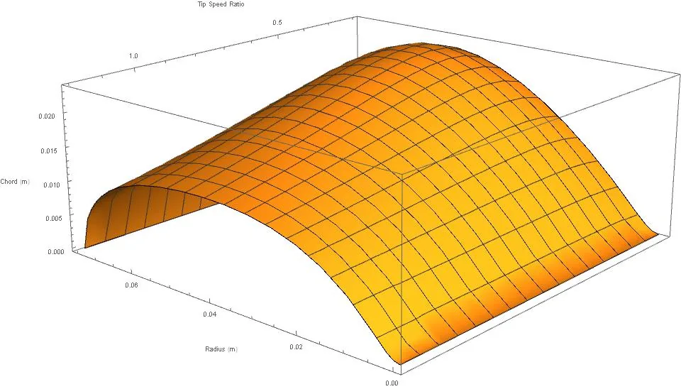
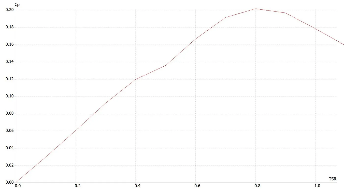
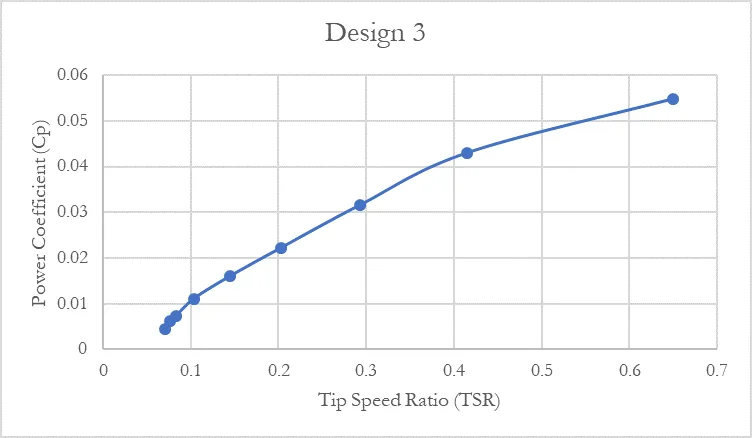
We assume that \(\lambda \approx 1\), as it was in the tests of our previous designs which maximized \(C_P\). Our final \(c(r)\) and \(\theta(r)\) are shown in Figure 6.
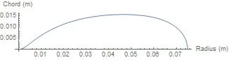
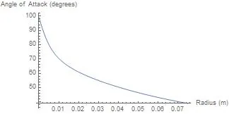
As QBlade's interpolation is only linear, I sample \(c(r)\) and \(\theta(r)\) at fifteen points and create fifteen cross-sections. The final rotor is shown in Figure 7.
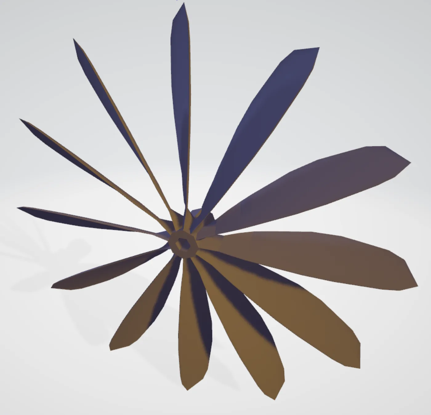
We can calculate the approximate swept area and rotor solidity by integrating the area of each blade (neglecting the effects of twist on the planform area of the turbine). After substituting the necessary constants, we have
\[\int_0^{0.075}\frac{14.8148 r \arccos(e^{-9.12 r })]}{\left(0.333 + 466.667 r+ \sqrt{1089.89 +r(311.111+217778 r)}\right)\left(\sqrt{0.444 +0.000204082\left(1-466.667r-\sqrt{1089.89+r(311.11+217778r)}\right)^2} \right)}dr\] \[=0.000884\] Multiplying by the number of blades, we find \[A_{swept} = 0.0106\] and solidity \[\sigma \approx 0.6\]
Results
Acknowledgments
I would like to thank Matthew for the help with my design and printing, Mike for his endless work and patience, and Prof. El-Gabry and the rest of the AIs for keeping the course interesting.
References
Jamieson, P (2018). Innovation in wind turbine design. London: Wiley.
Seelig, C (1960). Albert Einstein: a documentary biography. London: Staples Press.