The Eye
Before embarking on the design of a system located on, optically modifying, and intended to reckon the orientation of the eye, a basic understanding of the organ is necessary.
Anatomy
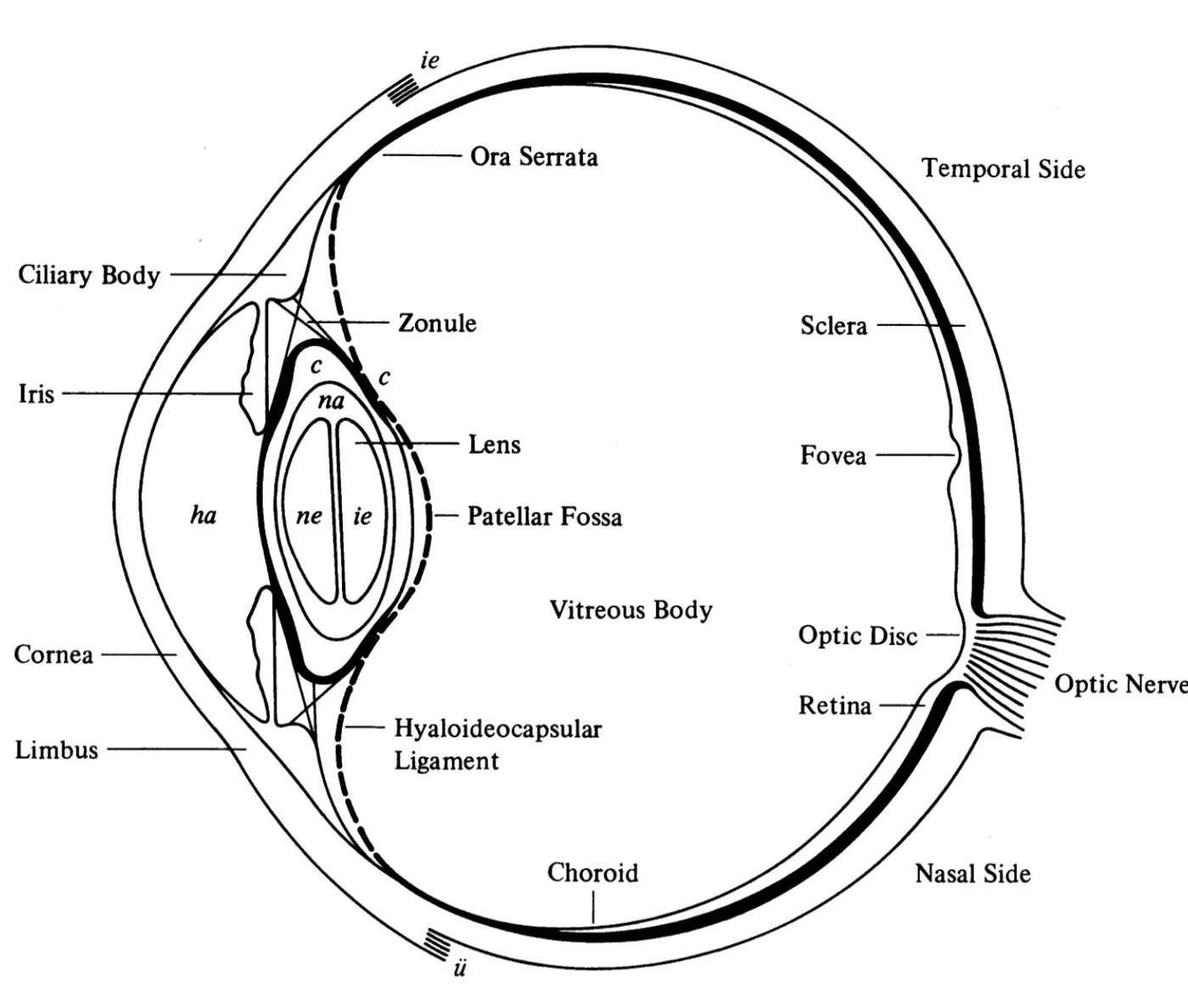
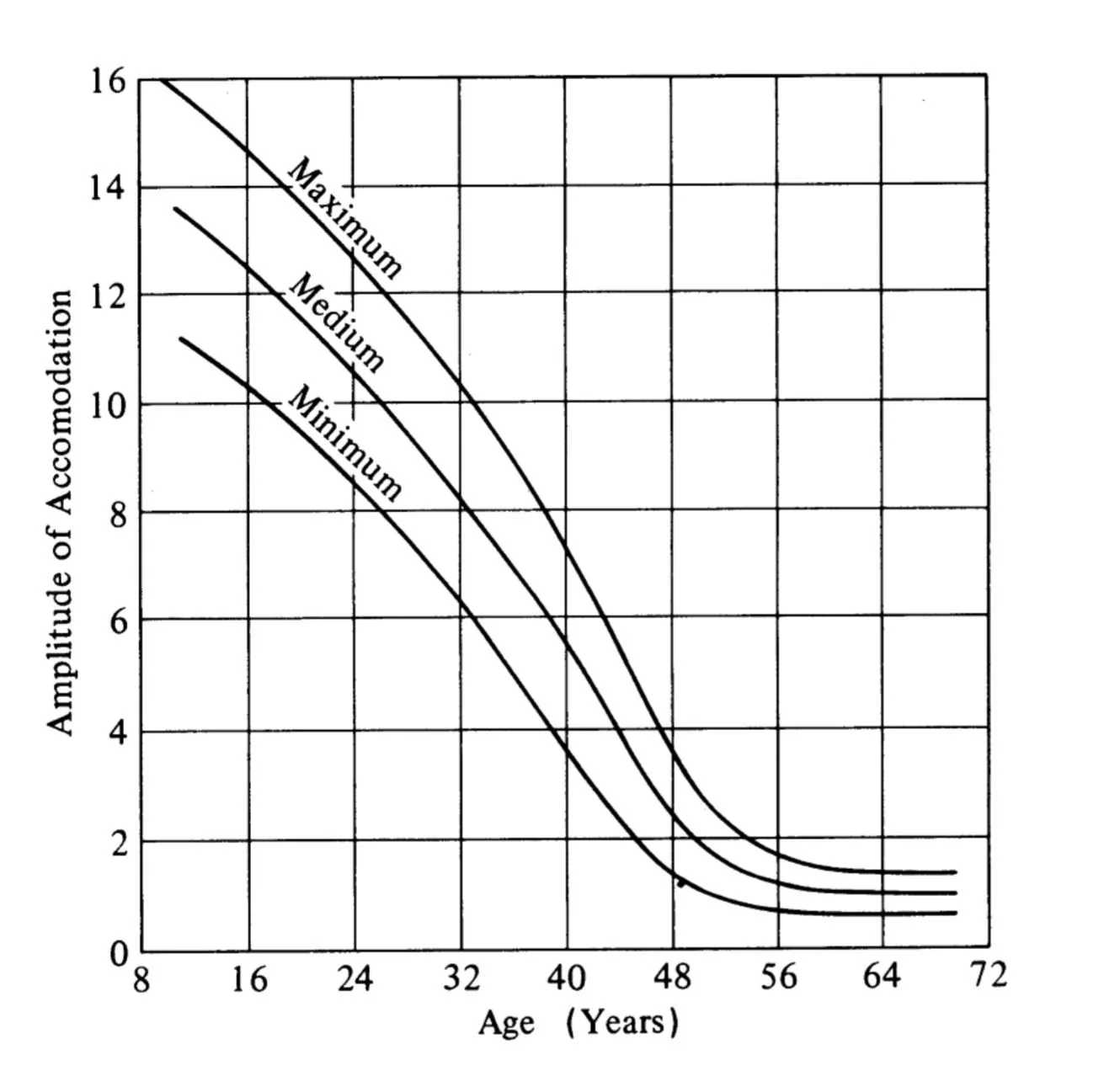
A top view of the eye is shown in Figure 1. The eye, as might be predicted by the size of its dedicated nerve, is a complex organ. The cornea, transparent, and sclera, opaque, form the outer surface of the eye. The cornea, covering the exposed area of the eye, is dense with nerve endings, six hundred times as many pain receptors as the skin, enabling the reflexive closing of the eyelid in response to slight variations in pressure, temperature, or chemical content. The cornea contains no blood vessels; oxygen and nutrients are delivered via diffusion in tears. Structures like contact lenses placed on the cornea must therefore be permeable to oxygen or largely physically detached as to permit tear flow. The outer layer of the cornea, the epithelium, becomes opaque when starved of oxygen, obscuring vision. The rest of the eye's encapsulation (approximately 5/6 area) is the white, fibrous sclera, which meets the cornea at the limbus. The pupil controls the amount of light that enters the eye, varying in diameter from 1.5 mm to \(\sim\)10 mm. Opaque elements of a contact lens must not intersect this area. Action of the pupil is closely related to that of the lens; the pupil's diameter decreases when the eye focuses on an object in the near field. The lens changes shape (accommodates) to focus the image on the retina. The lens never ceases developing, new layers deposited like the strata of an onion for the lifetime. Thickness increases by nearly 50% by 70 years of age, causing the lens to stiffen as it ages and reducing its accommodation range: presbyopia. Figure 2 details the deterioration in vision caused by presbyopia as a function of age.
The shape of the lens is altered by the ciliary body, a ring of muscles anchored by the zonules to the lens's equator. When the muscles of the ciliary body contract, the ring's diameter decreases and the lens thickens, providing near-field focus. Conversely, when the muscles relax, the ring's diameter increases and the lens flattens, providing far-field focus. The retina, atop the choroid and sclera, contains the eye's sensory cells. Those cells are concentrated about the fovea and absent at the optical disk, where the optic nerve exits the eye. Notably, the eye moves such that the fixation point is focused on the fovea, which is not geometrically centered in the eye: the geometric axis of the eye is distinct from its optical axis. Six muscles control each eye's movement, enabling changes in azimuthal angle \(\theta\)\(\theta\)azimuthal angular displacement, altitude angle \(\phi\)\(\phi\)altitudinal angular displacement, and torsion angle \(\zeta\)\(\zeta\)torsional angular displacement (rotation about the geometric axis).
Geometry and Movements
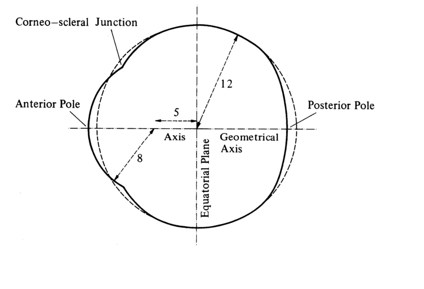
The average dimensions of the eye are labeled in Figure 3. Relevant to contact lens design are the radii of curvature of the cornea and sclera. Contact lenses, unless specially fitted, are designed to conform roughly to the geometry of the cornea and sclera. Just as tears render the cornea a near-perfect optical surface (regardless of the abnormalities in its structure), they fill any cavity between a lens and the surface of the eye. Contact lenses should be less than 250 \(\mu\)m, with a maximum diameter of 24 mm (scleral) or 12.5 mm (corneal), though these dimensions vary with wearer. As noted earlier, the geometric axis, passing through the center of the pupil and the center of rotation, does not intersect the fixation point because the eye centers the image on the fovea. The fovea is not co-linear with the center of rotation and center of the pupil. The eye rotates in three dimensions: an azimuthal rotation range of \(\theta \in [-44\pm7^{\circ}, 45 \pm7^{\circ}]\), where positive \(\theta\) is defined as rotation of the left eye from focus at infinity toward the nose (\(\theta_1\)) or of the right eye from focus at infinity away from the nose (\(\theta_2\)); an altitude rotation range of \(\phi \in [-47\pm8^{\circ},28\pm8^{\circ}]\); and a torsional range of \(\zeta \in [-8\pm2^{\circ},8\pm2^{\circ}]\). The eye rarely approaches the extrema of its range; movements of more than \(20^{\circ}\) in \(\theta\), for example, are usually supplanted by movement of the head. Mean interpupillary distance \(s\)\(s\)interpupilary distance, the distance between the geometric axis when the eyes are focused at infinity, is 62\(\pm\)3.6 mm for women and 64\(\pm\)3.4 mm for men. Geometric parameters of the eye vary by about 10% among individuals.
Though the eyes have three degrees of freedom, \(\zeta\) is entirely determined by \(\theta\) and \(\phi\), except when the eyes are presented images oriented at different \(\zeta\) angles (cyclodisparity), unusual in normal settings. Listing's Law, the exact functional relation \(\zeta(\theta,\phi)\), is simplest in quaternion or angle/axis representation: \(\zeta(\theta,\phi) = 0\). In other coordinate systems, the representation is more complex. A lucid explanation of Listing's law can be found in and a (intimidating) derivation in. As I was not able to incorporate torsional movement into my physical model, the first control models of Chapter 2 neglect torsion. In the control system incorporated into the lens, the angular position of the eyes might be represented in quaternions (more common than angle/axis in computation), as they require fewer computations than rotation matrices to determine the result of chained rotations (like the effect of incremental changes in \(\theta\) and \(\phi\)). Quaternion representation would also simplify the incorporation of Listing's law into the dynamics used to predict position.
At large angular amplitude, the eye engages in three distinct motions: tracking, vergence, and saccades. Tracking is movement of the eyes to maintain fixation on an object across the visual field. Tracking lasts seconds and rarely exceeds an angular speed of \(25^{\circ}/s\). Vergence, independent \(\theta\) changes of the eyes as to unify their fixation points (the eyes are spatially separated), are usually slow, \(\sim10^{\circ}/s\), but can reach angular speeds of \(200^{\circ}/s\). Saccades are rapid, simultaneous movements of the eye 20-200ms in duration with maximum angular speed of \(900^{\circ}/s\). Saccades occur when the eyes fixate on a new point in the visual field.
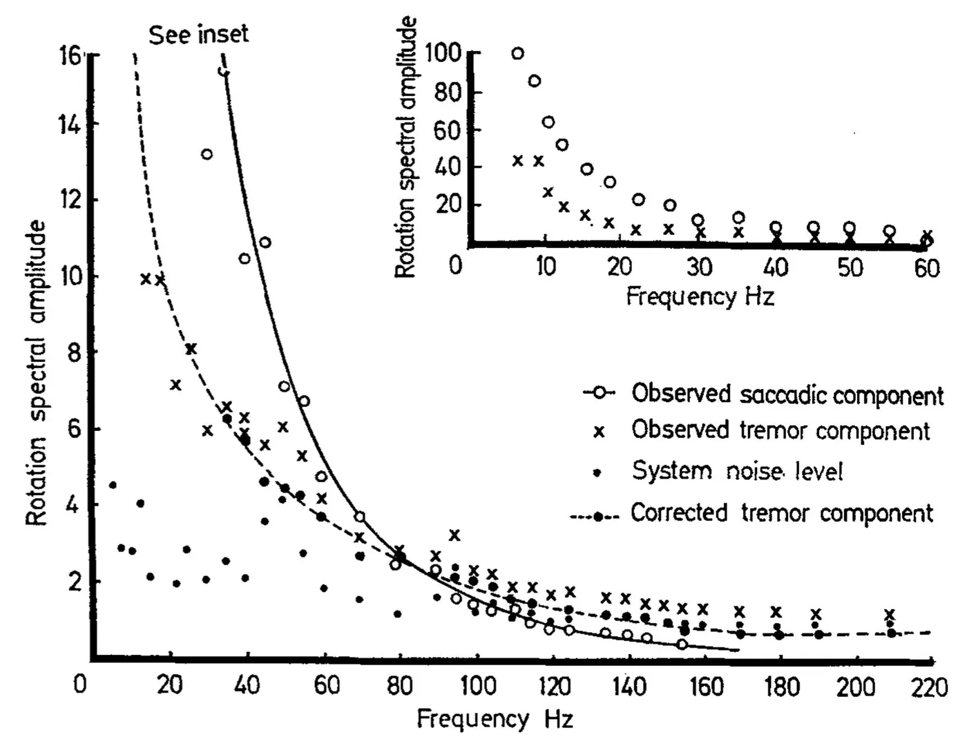
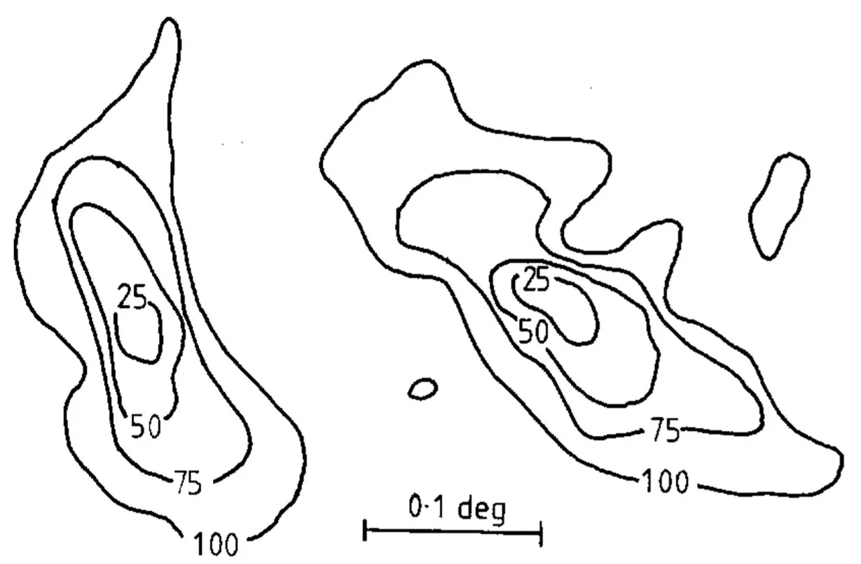
The eye also engages in angular movements of a scale several orders of magnitude smaller: tremor, drift, and microsaccades. Tremors occur at frequencies between 10 and 200 Hz (Figure 4) with magnitude \(\sim0.005^{\circ}\), drift movements at frequencies of about 1 Hz with magnitude \(0.03^{\circ}\) to \(0.08^{\circ}\). No correlation exists between the eye's drifts. Microsaccades, which correct displacements caused by drift, are not well characterized. The effect of these "miniature" movements is visible in Figure 5.
Besides geometric constraints dictated by the eye and the characteristics of its motion, we desire a relation between the \(\theta_i\) displacements and focal distance.
\(d\)distance from the observer to the fixation point: in a radial coordinate system with origin at the midpoint of eyes, the radial coordinate of the eyes' fixation point
\(d\)in a radial coordinate system with origin at the midpoint of eyes, the angular displacement of the fixation point from a ray perpendicular to the line between the eyes
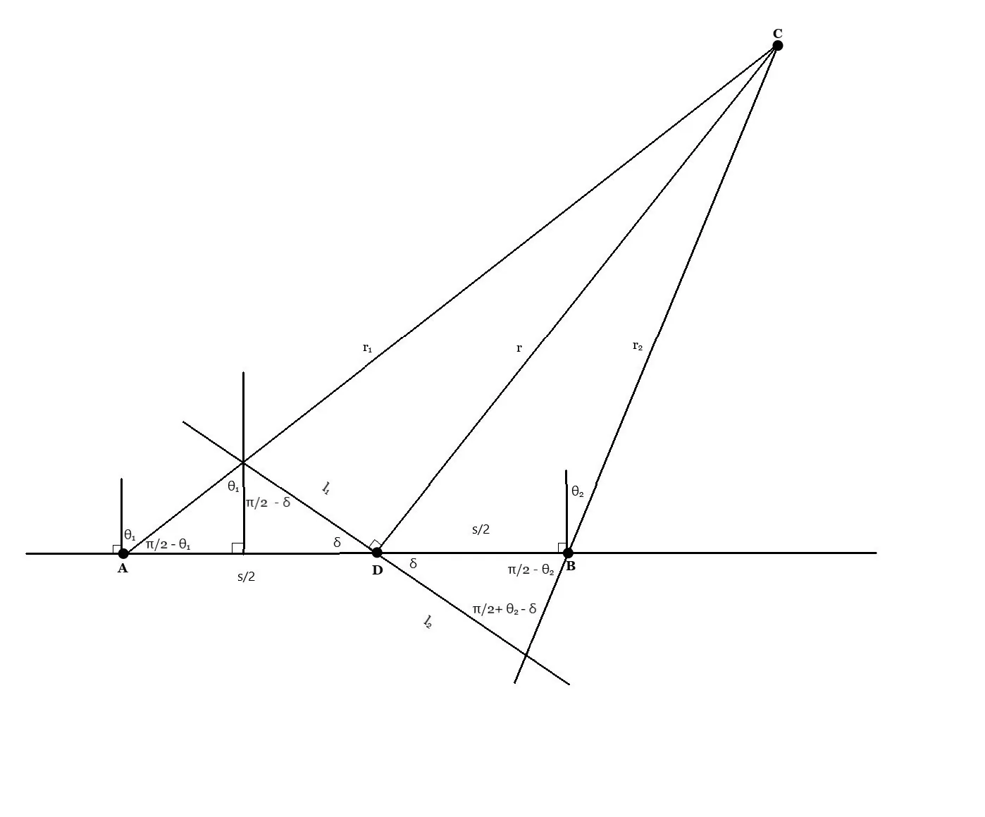
A and B are the centers of rotation of the left and right eyes, respectively, C is their fixation point, and D, midpoint of the \(\overline{\boldsymbol{\text{AB}}}\), the point from which effective fixation distance \(r = \overline{\boldsymbol{\text{DC}}}\) is measured. The accommodation of the eyes is not independent, strongly related to the vergence angle (\(\theta_d\)), fixation point distance (\(r_1\), \(r_2\)), and pupil diameter (pupil contraction for closer objects). for \(r>>s\), \(r \approx r_2 \approx r_1\). We first derive \(r(\theta_1,\theta_2)\), then \(r_1(\theta_1,\theta_2)\) and \(r_2(\theta_1,\theta_2)\).
When \(\delta = 0\), the length base of the triangle is determined, \(l_1 = l_2 = s/2\) and an expression for \(r\) is easy to compute:
For \(\delta \neq 0\), \(l_1 \neq l_2 \neq s/2\): determining \(r\) from only \(\theta_r\) is not possible. Rather, we try to compute an expression for \(r(\theta_1,\theta_2)\). Thinking of \(\overline{\boldsymbol{\text{AC}}}\) and \(\overline{\boldsymbol{\text{BC}}}\) as lines and defining our origin at D, we have: \[ y -y_1 = m(x-x_1)\]
and
Equating and solving for x,
Substituting back into either of our original equations for the lines ((2) or (3)),
because the origin of our coordinate system is the point at which \(r\) initiates,
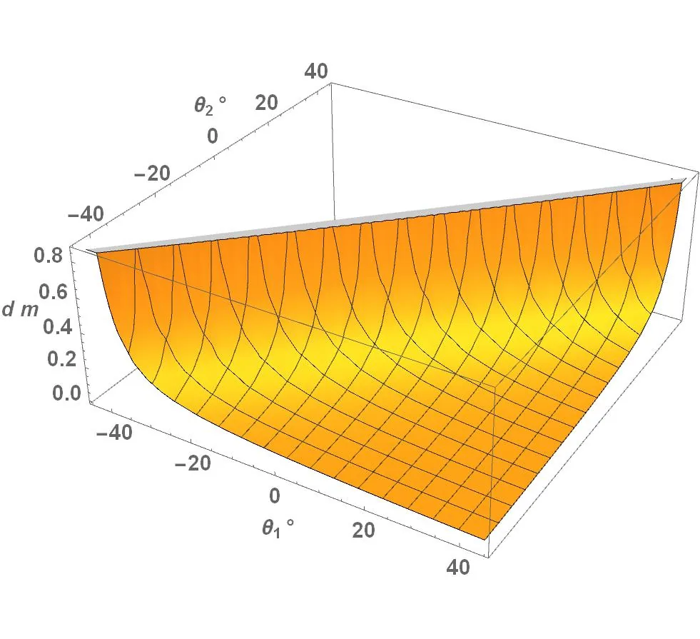
Results for \(r\) are presented in Figure 7 for \(\theta_1 \in [\theta_2,44^{\circ}]\), \(\theta_2 \in [-44^{\circ}, 44^{\circ}]\), \(s = 0.064 m\) as is characteristic in humans. As expected, the plot diverges in the limit \(\theta_1 \to \theta_2\): your eyes approach parallel as the distance to the fixation point increases.
We compute \(r_1(\theta_1,\theta_2)\) and \(r_2(\theta_1,\theta_2)\) by changing variables. First \(x \to x + s/2\):
Plugging back in,
so
\(d_2\) can be found by switching \(\theta_1\) and \(\theta_2\) and negating \(s\) (shifting the origin in the initial equations of the lines), yielding
We can compare these to the result we found for \(\delta = 0\).
and
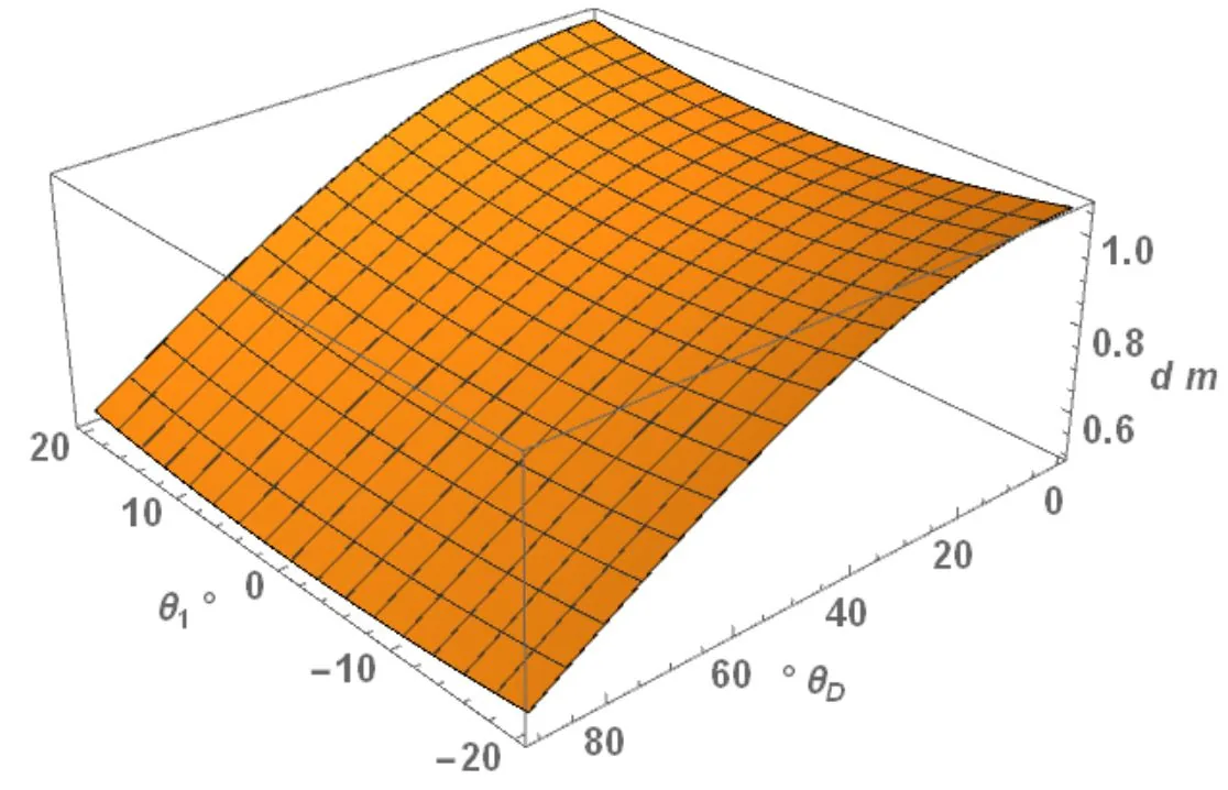
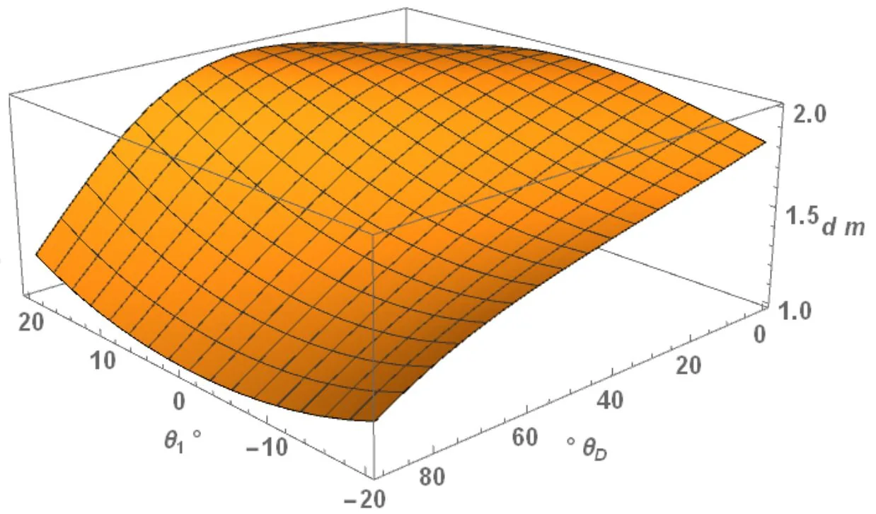
Equations 12 and 13 are plotted in Figures 8 and 9, respectively. Clearly, the models underestimate fixation distance in the near field and overestimate it at farther distances (the actual accommodation distance is some value intermediate between its distance from the origin of the primary coordinate system and its actual distance from the eye).
Optics
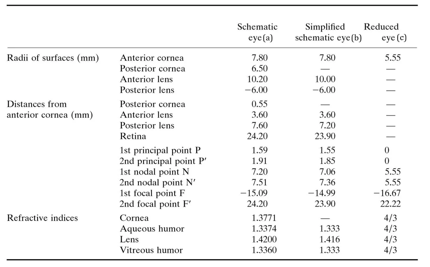
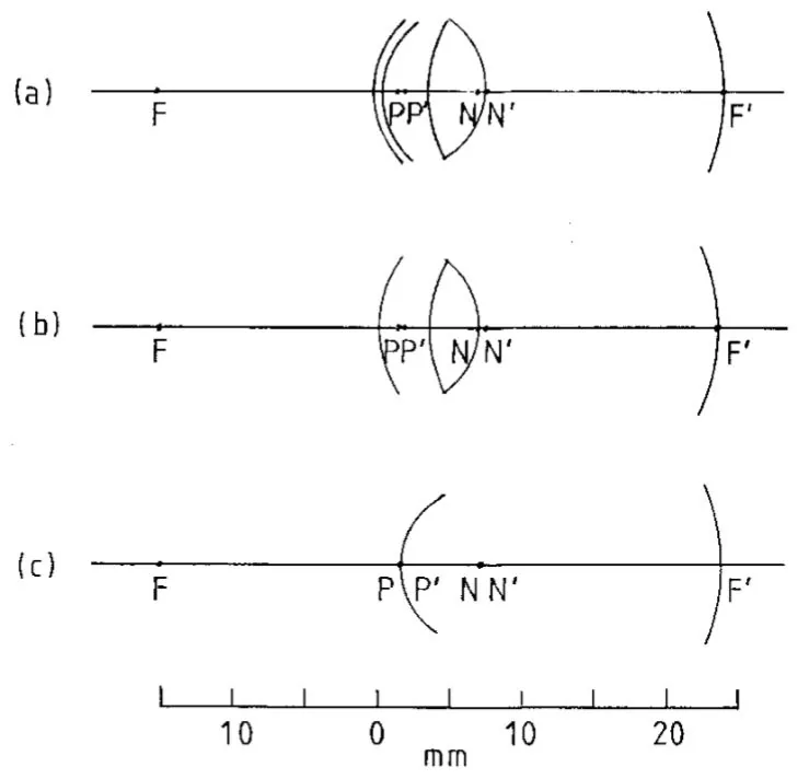
Several optical models of the eye exist, summarized in the table and diagram of Figure 10. Integrating a contact lens simply requires the addition of another optical element with a posterior radius and position equivalent to those of the posterior cornea. These models are easily instantiated in Zemax: see Chapter 3.
Control Systems
Because embedding of an LC lens in a contact lens will require nanofabrication of a lens, the training for which I have only partially completed (25 hours), and because lens design is highly sensitive to the performance of the yet undesigned power system, I begin by producing a control system. The control system can readily be modeled with commercially available components.
Measurements
Three measurements yield data sufficient to calculate the appropriate focus of an artificial lens for a presbyopic eye: fixation distance, accommodation, and vergence (Figure 11).
Power requirements of active sensors make direct measurements of the fixation distance impractical. Power delivery is limited by biological constraints on incident radiation and geometric constraints on the antenna (which must be embedded in a contact). High power use is usually also accompanied by heat, which is difficult to dissipate from such a small, biologically-mounted device. A LIDAR unit aligned with the optical axis might otherwise be the simplest method of measuring fixation distance.
Accommodation, the change in the focal length of the eye's natural lens, provides a natural control system for an artificial lens. The presbyopic eye attempts to achieve proper accommodation even when the necessary deformation of the natural lens is no longer possible (hence increased fatigue after unaided attempts to focus in the near field). An artificial lens might supplement natural accommodation by changing focal length until the natural lens is nearly relaxed. Were this the sole sensor input, however, the natural lens would never fully relax; otherwise, in steady state, the natural eye would focus at infinity (its maximum), making it impossible for the system to identify a subject's attempt to increase their focal length. Some measurement of accommodation will be required in an active contact lens such that the display projection system can remain focused on the retina. Accommodation can be determined via measurements of refractive changes (refractive power, negative spherical aberration) or of biometric changes (lens curvature, diameter, thickness). Devices for the measurement of all of these quantities exist for ophthalmologic purposes, though none on a scale suitable for the purposes of this project. Further research is required to determine which measurements might be completed from the platform of a contact lens.
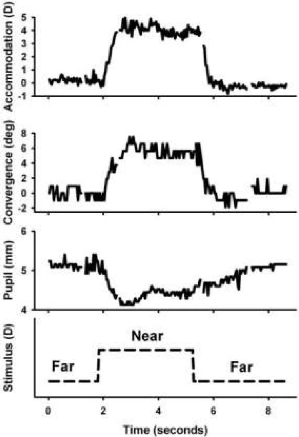
Vergence, the difference in lateral angle of the eyes, can be used to determine approximate fixation distance (via the Equation1). Currently, there exist no gyroscopes small enough to embed within a contact lens. Rather, as a contact lens is subject to torque (displaced from the center of rotation), an accelerometer might be used to dead reckon orientation. A control system based on accelerometers would not produce constant deformation of the lens (strain on the eyes). On long timescales, the mean and mode of an eye's orientation are directly forward (primary position), making such an estimate slightly more reliable. A control system based on vergence is easily manufactured (if not implemented in a lens); with this design my work shall begin. Accelerometers approaching the proper scale are available commercially: the MC3635 measures 1.6mm x 1.6mm x 0.94mm and produces 3-axis data. Besides system noise, the primary complication of a vergence-based control system is that communication between the sensors on both eyes is required. This, however, is a problem for Chapter 4. As the eyes are spatially separated, the system will eventually require two microcontrollers, each paired with a single accelerometer, communicating wirelessly. Wireless communication is difficult because there exist no Bluetooth or WiFi modules small enough to embed in a contact lens: the device's transceiver would need be designed for this purpose (in addition to power harvesting). Transceiver design is covered in Chapter 5.
Microcontrollers
Ideally, the system's microcontroller will be embedded in the contact lens. Designing a control circuit is far beyond my current electrical engineering abilities. Fortunately, much of the sensor and control suite can be modeled using commercially available components. Microcontrollers approaching the proper scale are available commercially. The Kinetis KL02, for example, measures 3mm x 3mm x 0.5mm, with 48MHz clock speed and 32kb flash. With a bit of grinding, the thickness might be reduced until embedding is possible. I begin by producing a system to measure vergence (requiring communication between the eyes), first implementing the system at a manageable scale with a Raspberry Pi and two relatively large sensors on a model eye system. If the larger system proves successful, I will produce the system at scale using the MKL02Z32VFM4 and MC3635.
Proof of Concept Control System
Producing a model with a Raspberry Pi and Adafruit accelerometers appears straightforward. Appearances can be deceiving. I begin with the simplest model possible: an accelerometer mounted on a single servo, intending to produce a model predicting absolute accelerometer position, to be compared to real servo position. Real servo position is measured using the servo's potentiometer, or, under minimal load (as in this design) estimated by empirically relating the servo input (duty cycle) and servo position. Internal to a servo is a control system that uses the device's potentiometer to precisely regulate motor position: duty cycle should map accurately to position. Unfortunately, the servo, removed from one of my model aircraft, was too imprecise, only responding to changes of duty cycle corresponding to angular changes of \(\sim5^{\circ}\). Accuracy, too, varied from my empirical fit (by as much as 10\(^{\circ}\)). More significant than servo misperformance, however, was the failure of the model to represent the problem. Error accrued in an accelerometer-based angular measurement system on the eye comes not only from sensor noise but external accelerations of the head and body, which cannot be consistently determined by a single accelerometer. (The gravitational vector \(\vec{g}\) can be used to compute the accelerometer's orientation. External accelerations make it difficult to determine \(\vec{g}\).) Additionally, a single eye's orientation has more degrees of freedom than the relative orientations of two eyes (the information we actually desire).
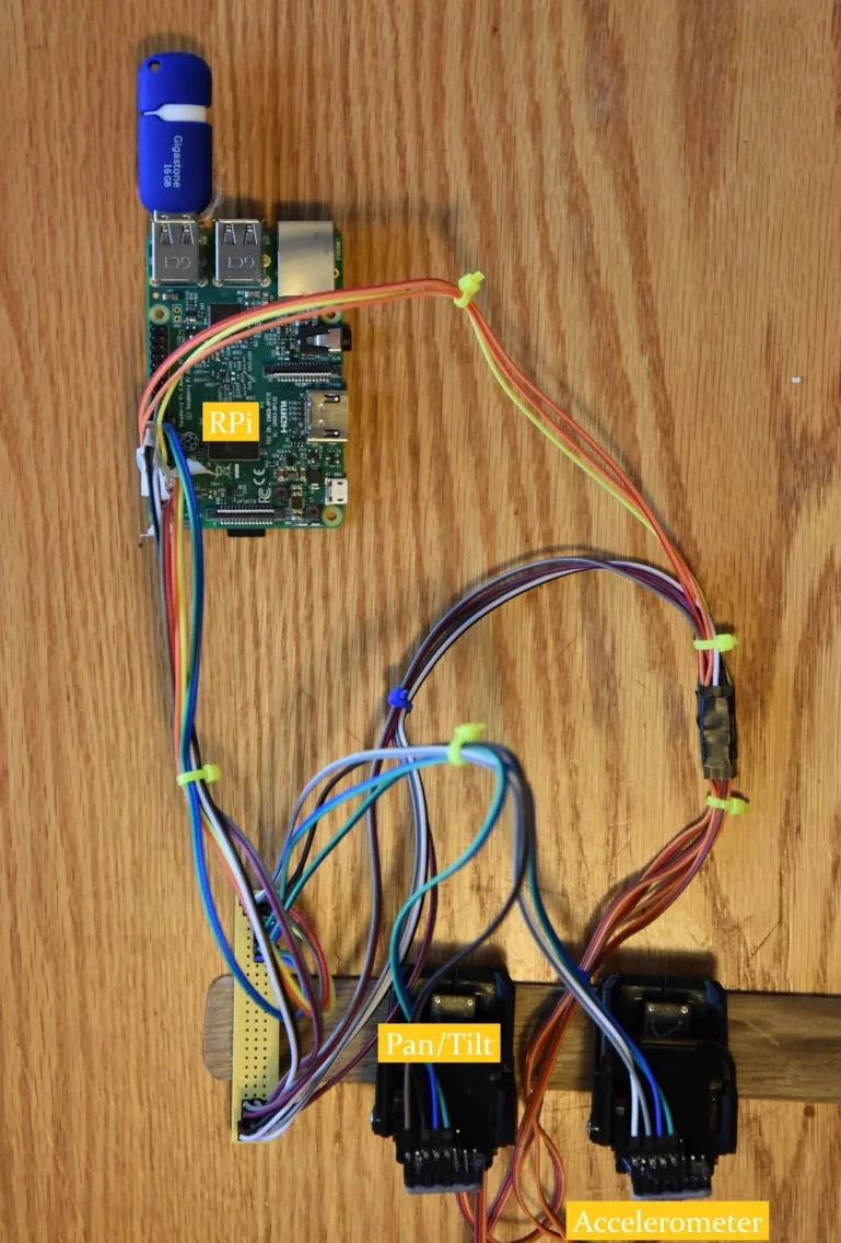
Two accelerometers, each mounted on a pan-tilt platform, comprise my second model (Figure 12). Except for torsion, all degrees of freedom of a natural eye are now represented: both azimuthal \(\theta\) and altitudinal angular motion \(\phi\) (Figure 13). Higher quality servos were used in the construction of the pan-tilt platforms in hopes of improving angular resolution. Worried about the performance of the physical model, I also produce a software model that produces the same output. It is easiest to understand both by first considering the software model, devoid of the peculiarities of the specific accelerometers and servos I used.
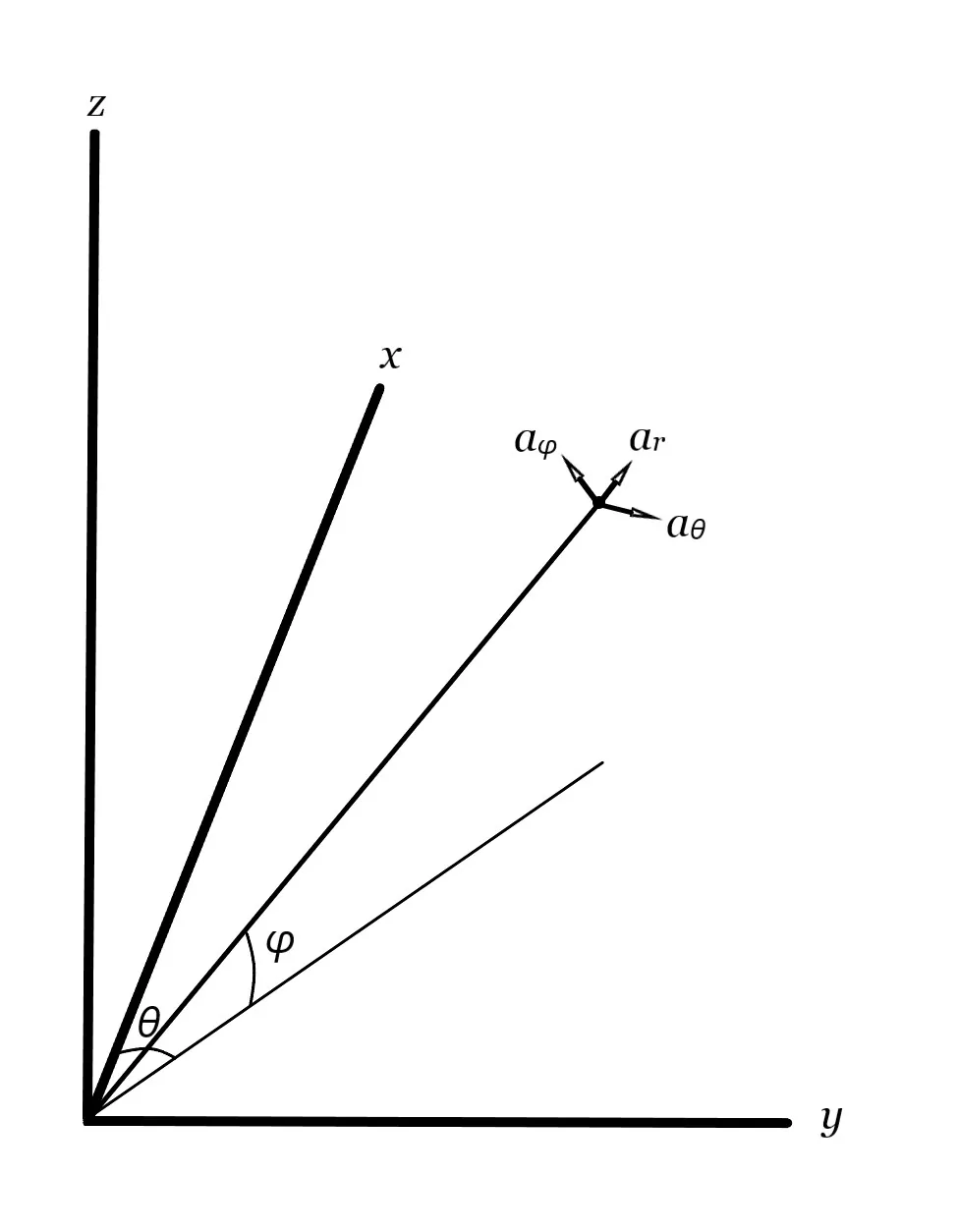
We begin by defining our coordinate system: Figure 13. Note that this is not the standard spherical system: altitudinal angle \(\phi\) is defined from the \(x-y\) plane and \(+y\) is defined in the opposite direction of normal (left handed), so as to correspond to the way we think: normal eye orientation corresponds to \(\phi=0\) and positive \(y\) and \(\theta\) to the right, from the observer's perspective. \(+x\) corresponds to forward to the observer and \(+z\) to upward from the observer's perspective. We use three reference systems in each model, the primary system, with origin at the midpoint of the geometric centers of the eyes (D in Figure 6) and coordinates \((x,y,z,r,\theta,\phi)\), the left eye coordinate system, with origin at the geometric center of the left eye (A in Figure) and coordinates \((x_1,y_1,z_1,r_1,\theta_1,\phi_1)\), and the right eye coordinate system, with origin at the geometric center of the right eye (B in Figure 6) and coordinates \((x_2,y_2,z_2,r_2,\theta_2,\phi_2)\). \(r, r_1, \theta_1, r_2\), and \(\theta_2\) are labeled on Figure 6.
Conversions between Cartesian and spherical in this coordinate system are
and
Spherical velocity is given by
and acceleration by
Geometrically, the program accepts a paramaterized position and computes the \(\theta\) and \(\phi\) coordinates of a ray from the geometric center of each eye to that point as a function of time. It then calculates the first and second time derivatives of those coordinates, which it uses to compute the velocity and acceleration of a point with radius R_EYE. After the addition of some Gaussian noise, the necessary outputs are computed over the time vector and returned. More specifically, the software model Simulation_Artificial.py accepts the variance of the sensor's static measurements, the parameterized location of the fixation point as a function of time, and the duration of the simulation, returning a matrix of orientation data containing the time, Cartesian location of the fixation point in the primary coordinate system, and orientation of the right and left eyes; a matrix of acceleration data containing the time and three-dimensional acceleration of each eye; a vector of the variance of the sensor's static measurements (to reproduce the output of the physical model); and a matrix of the initial orientations, velocities, and accelerations.
Starting with the parameterized position,
x = f(ts)
                y = f(ts)
                z = f(ts)
we convert to right and left eye coordinate systems (a shift in y)
y1 = y - SEPDIST/2.0
                y2 = y + SEPDIST/2.0
and find the spherical position in those coordinate systems (Equation 14)
theta1 = atan(y1/x)
                phi1 = atan(z/(x**2+y**2))
                theta2 = atan(y2/x)
                phi2 = atan(z/(x**2+y2**2))
The computation now bifurcates depending on our desired acceleration output. In the physical model, the accelerometers produce \((a_r,a_{theta},a_{phi})\) data. Spherical data is difficult to work with. For example, numerical integration of spherical data is possible in \(\theta\) and \(\phi\), but not \(r\). Total spherical integration requires linearization in an extended Kalman filter, while Cartesian (and \(\theta\) or \(\phi\)) integration requires only a Kalman Filter. For the purposes of comparing different position estimation techniques, we therefore also produce Cartesian data (as might be produced by an accelerometer whose orientation with respect to the \(x\), \(y\), and \(z\) axis is fixed). To produce spherical data, we differentiate twice (computing velocity to allow calculation of the initial state)
avtheta1 = diff(theta1,ts)
                avphi1 = diff(phi1,ts)
                avtheta2 = diff(theta2,ts)
                avphi2 = diff(phi2,ts)
                aatheta1 = diff(avtheta1,ts)
                aaphi1 = diff(avphi1,ts)
                aatheta2 = diff(avtheta2,ts)
                aaphi2 = diff(avphi2,ts)
use Equations 16 to calculate velocity
r = R_EYE
                vr1 = 0
                vtheta1 = r*avtheta1*cos(phi1)
                vphi1 = r*avphi1
                vr2 = 0
                vtheta2 = r*avtheta2*cos(phi2)
                vphi2 = r*avphi2
and Equations 17 to calculate acceleration
ar1 = -r*(avtheta1*cos(phi1))**2-r*avphi1**2
                atheta1 = r*aatheta1*cos(phi1)-2*r*avtheta1*avphi1*sin(phi1)
                aphi1 = r*avphi1**2*sin(phi1)*cos(phi1)+r*aaphi1
                ar2 = -r*(avtheta2*cos(phi2))**2-r*avphi2**2
                atheta2 = r*aatheta2*cos(phi2)-2*r*avtheta2*avphi2*sin(phi2)
                aphi2 = r*avphi2**2*sin(phi2)*cos(phi2)+r*aaphi2
We construct the position, base acceleration, and initial state matrices by inputting the time vector t
abase = np.vstack((ar1(t), atheta1(t), aphi1(t), ar2(t), atheta2(t), aphi2(t)))
                orientation = np.vstack((t,x(t),y(t),z(t),theta1(t),phi1(t),theta2(t),phi2(t))).transpose()
                s0 = np.array([[ R_EYE,  theta1(0),  phi1(0),  R_EYE,  theta2(0),  phi2(0)],
                               [   vr1, vtheta1(0), vphi1(0),    vr2, vtheta2(0), vphi2(0)],
                               [ar1(0), atheta1(0), aphi1(0), ar2(0), atheta2(0), aphi2(0)]])
and add Gaussian noise to the acceleration to reproduce accelerometer data (D is the number of dimensions of the measurement, 6 in this case)
anoise = np.zeros((D,len(t)))
                for i in range(D):
                    anoise[i,:] = np.random.normal(scale = np.sqrt(avar[i]), size = len(t))
                acceldat = np.vstack((t, abase + anoise)).transpose()
The procedure for Cartesian acceleration is similar: we compute expressions for the Cartesian location of points at radius R_EYE (x1, y1, z1, x2, y2, z2), differentiate twice, compute orientation, base acceleration, and initial state matrices, and add acceleration noise. However, the variance of noise in each dimension now fails to correspond to accelerometer variance (spherical) on any axis, so we assume that variance is equivalent in all axes to the mean of the accelerometer variance matrix, reasonable as the accelerometers we use in each dimension are identical, each with variance \(\sim 0.005 m/s^2\).
The physical model takes as input desired motion type movetype–varying \(\theta_d\), \(\theta_d\) and \(\theta\), \(\theta_d\) and \(\phi\), or \(\theta_d\) and \(\theta\) and \(\phi\)–and the number of iterations (iterations) of that motion to complete and produces as output accelerometer measurements, accelerometer variance, and intermittent orientation data (except initial state output, identical to the software model). Software for the physical model consists of three files. Acclerometers.py begins by initializing the accelerometers. Assuming the sensors are initially at rest, it reads several thousand samples of raw data, normalizing it (with respect to \(\vec{g}\)), and calculates each accelerometer's variance. The class's other function then produces acceleration data using the initial normalization. Servos.py initializes the servos, setting up PWM on the correct GPIO pins, and rotating them to primary position. The class also contains functions to rotate servos individually or simultaneously to particular angles and to rotate them such that the pan-tilt platform fixates on a particular point (specified in the primary coordinate system). Finally, Simulation_Model.py produces accelerometer and servo objects, begins reading accelerometer data, and sends the servos to a sequence of iterations random fixation points in the subspace dictated by movetype. Specifically, after creating a Simulate_Model object, running the simulate(movetype, iterations) creates two empty arrays
acceldat = np.array([]).reshape(0,7)
                orientation = []
and a thread for servo movements (of type movetype)
mvservthrd = threading.Thread(target=wrapper, args=(movetype, (iterations,), orientation))allowing simultaneous direction of the servos and recording of data. We record the start time
t0 = t.time()begin the treading
mvservthrd.start()and start recording acceleration data, calling the acceleration function a on our accelerometer object a, rearranging to match our acceleration data format, and appending to the acceleration data array acceldat
while mvservthrd.is_alive():
                    ta = self.a.a()
                    ta = np.hstack((ta[0,:],ta[1,:]))
                    acceldat = np.vstack((acceldat,np.hstack((t.time()-t0,ta))))
when the sequence of servo movements finishes, we join the thread
mvservthrd.join()and return the data.
An example movetype is vergewtwj: vergence with \(\theta\) with jitter (\(\phi\)). I denote \(\phi\) movements jitter because they are poor representations of the movements of the eye: in the physical model, the axis of \(\theta\) and \(\phi\) motion are spatially separated by 20 mm (dictated by the design of the pan-tilt platform), while those in the eye are separated by less than 1mm. The spatial separation amounts functionally to an irreconcilable difference in the radius of rotation in \(\theta\) and \(\phi\). As we are primarily concerned with vergence (movements in \(\theta\)), I set the radius of \(\theta\) rotation to 14 mm, the average radius of the eye. This forces a \(\phi\) radius of 34 mm. The \(z\) magnitude of a \(\phi\) movement of the eye can be reproduced by corrective coefficient to the angle of rotation, but the corresponding movements and therefore accelerations in \(x\) or \(r\) are incorrect. I therefore limit movements in \(\phi\) to small magnitude displacements: jitter.
Again, we begin be creating a data array and recording the initial time
data = np.array([]).reshape(0,8)
                t0 = t.time()
Then iterations times, we generate a random fixation point in primary spherical coordinates within physiological bounds of \(r\) and \(\theta\) and at small \(\phi\) (jitter)
for i in range(0,iterations):
                    # focal distance
                    r = MIN_F_DIST + np.random.random()*(MAX_F_DIST-MIN_F_DIST)
                    # azimuthal
                    theta = (MIN_AZM_ANG + np.random.random()*(MAX_AZM_ANG-MIN_AZM_ANG))*DEGREES
                    # jitter, does not correspond to phi unless axis of z and y rot aligned in x
                    j = (MIN_J + np.random.random()*(MAX_J-MIN_J))*DEGREES
We then convert the position to primary Cartesian coordinates and use the to function of the servo class to rotate them such that the pan-tilt platforms focus on that point. The to function also returns the \(\theta\) and \(\phi\) angles of the fixation point in the right and left eye coordinate systems: the final orientations of the pan-tilt platforms. This is precisely the data required by our orientation matrix convention. Finally, we append the elapsed time t.time-t0, the Cartesian position of the fixation point in the primary coordinate system, and the orientations to our data array, which return upon the completion of iterations iterations of the loop. The servo's velocity and acceleration cannot be controlled, only its final position, so when the platform reaches the desired orientation, we collect data, wait a half second, and collect another row of data.
for i in range(0,iterations):
                    #convert to position of focal point
                    x = r*np.cos(j)*np.cos(theta)
                    y = r*np.cos(j)*np.sin(theta)
                    z = r*np.sin(j)
                    spherical =  self.s.to(x,0,z)
                    # focus on that point, wait a bit, recollect data
                    # so there is a flat bit with which to compare acc data
                    data = np.vstack((data,np.hstack((t.time()-t0,x,0,z,spherical))))
                    t.sleep(0.5)
                    data = np.vstack((data,np.hstack((t.time()-t0,x,0,z,fd,spherical))))
                return data
Between for the time interval each of these pairs of points sharing orientation and fixation point, we know position, velocity, and acceleration. Our knowledge of these intervals allows us to quantify the accuracy of orientation estimation algorithms.
The production of acceleration and orientation data with our software and physical models is only to test the accuracy and relative performance of our orientation estimation algorithms.
Though, having measured acceleration from the surface of both eyes, we might expect to be able to compute their absolute orientations, we can only realistically compute their relative orientation. The eyes are subject to the external accelerations of the head and the head to external accelerations of the body, accelerations of far greater magnitude than a \(10^{\circ}/s\) vergence movement of the eye. However, most external accelerations are consistent among the eyes: movements of the body, certainly, but also \(\theta\) and \(\phi\) movements of the head (defined from the center of the head's rotation). \(\zeta\) rotations of the head are largely negated by \(\zeta\) rotations of the eye. Even within the eye, motion in \(\phi\) (from the eye's geometric center) is largely coordinated. The difference in the acceleration experienced by the eyes, then, should mostly consist of the differences in their \(\theta\) accelerations. Alternatively, when integrated, the difference in the eye's absolute orientations should map well to their \(\theta_d\).
The task of orientation estimation, then, is accurate integration of the accelerometer data, perhaps after some preprocessing to remove sensor noise. We then might detrend the data over a window during which we expect eye position or velocity to have some predictable mean. I compare the results of trapezoidal integration and integration by Simpsons Method (with and without preprocessing) to the predictions of a Kalman filter. Trapezoidal integration linearly fits adjacent data points, and computes sum of the areas of the resulting trapezoids. Simpsons method is slightly more accurate; it quadratically fits each triplet of points, the areas of which it sums. The Kalman filter performs only basic numerical integration but accounts for Gaussian noise; in models where error results primarily from sensor noise rather than integration error (if sampling rate is sufficiently high or sensor variance of sufficient magnitude), we might expect the Kalman filter to outperform conventional integration. Note that the Kalman filter can only be applied in the \(\theta\) and \(\phi\) dimensions of spherical data. I also examine the effects of detrending of velocity intermediate in integration.
All of my completed position estimation functions are contained in PosEst.py. All of my integration methods take as arguments acceleration and initial state matrices formatted per my array conventions (see General.py) and return orientation matrices.
Trapezoidal integration is the simplest; opportunely, scipy contains a function for cumulative trapezoidal integration. I begin by extracting the time vector from the acceleration matrix and eliminating that vector from the matrix
acct = a[:,0].reshape(a.shape[0],1)
                a = a[:,1:7]
I then cumulatively integrate, adding vectors from the initial state as required
veltrap = integral.cumtrapz(a, acct, axis = 0, initial = 0)
                # add the initial velocity
                veltrap = veltrap + s0[1,:]
                postrap = np.hstack((acct,integral.cumtrapz(veltrap, acct, axis = 0, initial = 0)))
                # add intial position
                postrap[:,1:7] = postrap[:,1:7] + s0[0,:]
finally, if the integral is being performed in spherical coordinates, some additional work is necessary. The integration in r is invalid. We therefore set the \(r\) vectors to \(\vec{0}\). Integration can be performed in \(\theta\) and \(\phi\). Crucially, however, \(a_{\theta} \neq \ddot{\theta}\) \(a_{\phi} \neq \ddot{\phi}\) (see Figure 13). The result of integrating \(a_{\theta}\) or \(a_{\phi}\) is the arclength \(s\) of the path followed by a point undergoing those accelerations at fixed radius. But \(s=r\theta\) so \(\theta = \frac{\iint \ddot{\theta} \,dt\,dt}{s}\) (the previous relations also hold for \(\phi\)).
if(IF_SPH):
                    postrap[:,2:4] = postrap[:,2:4]/R_EYE
                    postrap[:,5:7] = postrap[:,5:7]/R_EYE
                    postrap[:,1] = postrap[:,4] = np.zeros(postrap.shape[0])
if the integration is performed in Cartesian coordinates, I convert to spherical before returning
else:
                    postrap[:,1:4] = spherical(postrap[:,1:4])
                    postrap[:,4:7] = spherical(postrap[:,4:7])
                return postrap
All integration outputs are in (left and right eye) spherical coordinates. The process for integration with Simpson's method is virtually identical, except that there are no preexisting cumulative options. I produce a function cumulative which integrates iteratively, and, as the process is computationally taxing, another that integrates iteratively only over a window preceding the data point of interest (uses the data point window size points prior as an initial value) optcumulative, which produces very similar results.
The Kalman filter is the optimal form of estimation when measurements are subject to Gaussian noise. A Kalman filter also "learns" relationships between elements of its state vector, the similar movement of each eye in \(\phi\), for example. The Kalman filter assumes state equations of the form
in which \(\boldsymbol{x}\) is the hidden (full) state and \(\boldsymbol{z}\) the observed state. The inputs of a Kalman filter are the transition matrix \(\boldsymbol{A}\), observation matrix \(\boldsymbol{C}\), transition covariance \(\boldsymbol{Q}\), observation covariance \(\boldsymbol{R}\), transition offsets \(\boldsymbol{b}\), observation offsets \(\boldsymbol{d}\), initial state mean \(\boldsymbol{\mu_0}\), and initial state covariance \(\boldsymbol{\Sigma_0}\) and returns for each timestep an updated state covariance and state mean (our output).
For each dimension, the elements of our state vector are
Our total state vector in Cartesian is then
or
in spherical. Our transition matrix for each dimension of each accelerometer is
so our full transition matrix \(\boldsymbol{A}\) is a block diagonal of the number of dimensions being measured, six for Cartesian and four for spherical. In spherical, we divide the results of position integration by R_EYE after filtering; incorporation of the division in the transition matrix (specifically, setting \(\boldsymbol{A_d[0,0]}\) to a value other than one) causes the algorithm to diverge.
Our observation matrix \(\boldsymbol{C}\), when multiplied by the state vector produces an array with the measurements on the diagonal. In this case the measurements are the acceleration in each dimension, so the array is 6x18 in Cartesian and 4x12 in spherical, with every third column equivalent to a column of \(\boldsymbol{I_6}\) or \(\boldsymbol{I_4}\). For example, in spherical,
The model covariance \(\boldsymbol{Q}\)–a quantification of our confidence in our model–we initialize to relatively small values: \(\boldsymbol{C} = 0.01*\boldsymbol{I_{18}}\) in Cartesian or \(\boldsymbol{C} = 0.01*\boldsymbol{I_{12}}\) in spherical. (small variance equates to higher confidence). Presumably the Kalman integration is relatively accurate so the real and simulated accelerometer readings map well to actual position.
The observation covariance \(\boldsymbol{R}\) we initialize to an array empty but for our accelerometer variances on the diagonal. None of our sensors are linked.
In our model, the transition offsets \(\boldsymbol{b}\) and observation offsets \(\boldsymbol{d}\) both equal \(\vec{0}\): integration is a function only of the acceleration, velocity, and position of the previous timestep, and our observations are exactly those accelerations of our state vector. Neither require the addition of constant offsets.
The initial state mean \(\boldsymbol{X_0}\), our estimate of the model's initial state is just the data of s0, a 3x6 or 3x4 matrix for Cartesian and spherical, respectively, reshaped as to correspond to our state vector (18x1 or 12x1).
Of initial state covariance \(\boldsymbol{\Sigma_0}\) we can only fill in the values of accelerometer variance accurately. We initialize it to an 18x18 (Cartesian) or 12x12 (Spherical) array of zeros and insert the relevant accelerometer variance at every third position along its diagonal.
We can begin by characterizing the different estimation models when fed data from the accelerometers at rest (noise alone). I configure the accelerometers for maximum performance: 12 bit data output at a frequency of 1344 Hz, \(\sim\)1kHz after accounting for the time required to record the data. I set the data output of the software model to the same frequency. Physical accelerometer variance is consistently \(\sim 0.005 m/s^2\) in each dimension; this I use to set accelerometer variance in the software model. At rest in either model (when stationary, we can eliminate \(\vec{g}\) in the physical model), we obtain results similar to Figure 14 for absolute position.
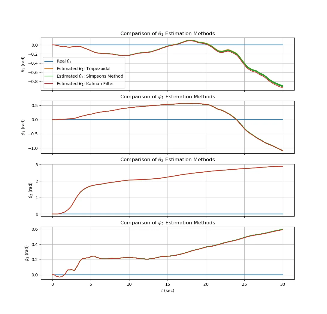
At rest, all estimations methods are virtually identical–our data is collected at high enough frequency that the integration method is irrelevant. The estimations, however diverge significantly from actual values. The problem compounds itself when we compute relative positions because the effect of the variances on the integration add.
I now try preprocessing of the data. Unfortunately, vergence movements are not periodic and have essentially no distinguishing velocity behavior (angular velocities of \(\sim10^{\circ}/s\) to \(200^{\circ}/s\), as stated in Chapter 1) by which they may be isolated. I can try, however, to eliminate some of the accelerometer noise. Applying a Savitzky-Golay (low pass) filter to the data of Figure 14, I obtain results almost indistinguishable from those of 14 except for some elimination of noise in Simpson's method (a result of Simpson's method's ability to compute integrals over odd numbers of data points). I therefore desist from preprocessing attempts.
Deviation of the estimates from actual orientation is strongly related to accelerometer variance, which contributes much of the noise. Nevertheless, we are unlikely to find accelerometers that perform significantly better than these as we require minute size. The divergence of the orientation estimates for stationary accelerometers therefore indicates that acceleration data alone is insufficient to produce a control system for our autoaccommodating lens.
We can now demonstrate the accuracy of relative orientations as compared to absolute orientations. In the software, subjecting the accelerometers to a constant \(z\) acceleration of 0.01 m/s, our absolute positions, become, for example, Figure 15
while our relative positions remain much closer to actual relative position.
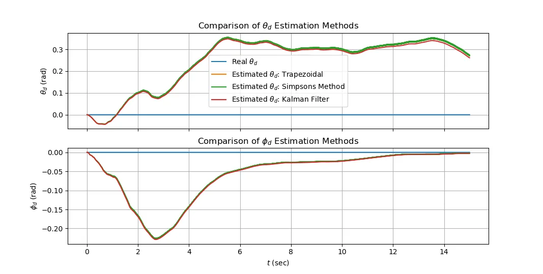
Next, we incorporate movement. Our physical model, designed specifically for the purpose of generating this data, fails us at this point. Again, the servos have frustratingly low accuracy (\(\sim 10^{\circ}\)). We turn to the software model for support. Setting the fixation point on the trajectory
x = 0.5*cos(3*ts)+0.51
                y = sin(3*ts)
                z = cos(3*ts)
we compare the performance of the various integration methods (Figures 17 and 18)
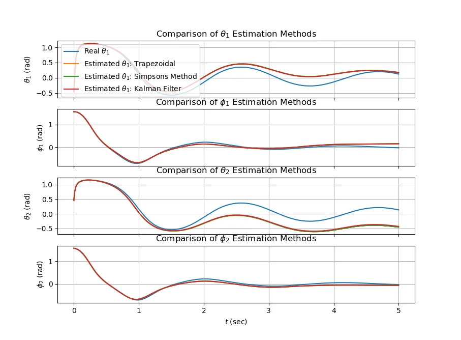
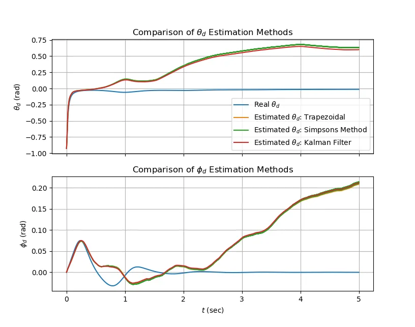
Again, the integration methods are essentially indistinguishable and diverge so rapidly from actual orientation or relative orientation as to make a control system based solely on accelerometer inputs impossible.
Finally, desperate, we add velocity detrending. Over a period as long as thirty seconds, we expect an average angular velocity in each dimension of approximately zero; while the eye's mean position might not be primary position over such an interval (while reading, or looking sidelong at a lecturer), the eye's range of rotation is sufficiently limited that angular velocity should be so slow as to be negligible or have mean zero. I use the scipy function detrend to shift the velocity data such that it has mean zero. On stationary position data, this does little, as the mean velocity is already zero, but on data with movement, it has better effects. Detrending the same data as Figure 18 yields the orientation estimates of Figure 19.
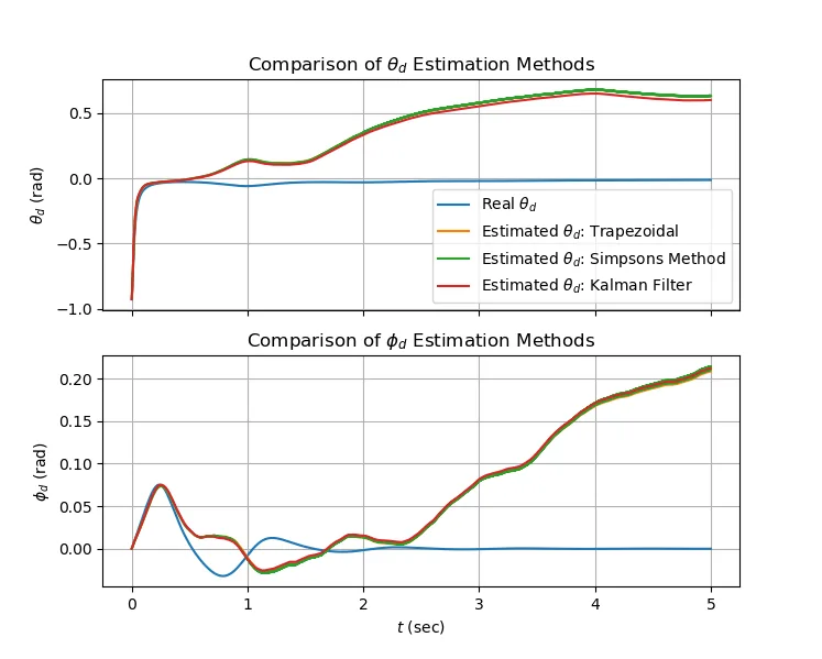
A slight increase in performance. It seems, regardless of the tools we apply to the task, calculating orientation from a noisy sensor's readings of the minute accelerations (in an environment of accelerations many orders of magnitude larger) cannot be done reliably.
Progress Summary and Future Work
Intending to produce a control system for an autoaccommodating lens, I tried to measure vergence using accelerometers mounted within the lens. I computed the relations by which vergence might be transformed into the focal distance required of the lens. I then produced two physical models and one software model of the accelerometer system to test the concept. Using a filtering, a variety of numerical integration techniques (including a Kalman filter), and demeaning, I attempted to extract the relative orientation of the eyes from acceleration data. The task proved impossible; the magnitude of sensor noise was too high. Though the idea of using accelerometers to recover orientation data from which accommodation might be controlled was a failure, the process was not. Before this project, I had never used Python, encountered Kalman Filters, or set foot in a clean room. I am now far more comfortable with each. And though this method of calculating orientation failed, the project's fundamental idea, an autoaccommodating lens, is unmarred. I need only devise a better sensor suite for control. I will begin with photodetectors. Placed in linear arrays radiating outward toward the nose and ear on the lens, they should be capable of measuring \(\theta_1\) and \(\theta_2\); when the eye rotates, some of them rotate under the skin. Simultaneously, I will begin producing variable focus LC lenses in the PRISM; I have already met with the lab staff to coordinate this work. The next semester looks exciting!
Liquid, hydrodynamic, hydraulic, and liquid crystal (LC) tunable lenses have been prototyped. LC lenses are optimal for this application. Constraints on the mass, volume, and speed (of focus) of the lens mechanism reduce applicable tunable lens technologies. A contact lens is subject to accelerations produced by the human eye, notably, saccade and version. Accelerations of \(\sim1m/s^2\) have been recorded, as well as accelerations of the head and body. Liquid lenses, in which the lens geometry is produced by electric or thermodynamic manipulation of the interface between two immiscible liquids, and hydrodynamic lenses, in which the lens geometry is produced by control of fluid flow patterns, are unsuitable to loading or acceleration of any type and therefore for this application. Hydraulic lenses, in which the lens geometry is produced by the variation of the pressure of fluid within a distensible membrane, have been used in prototypes of variable-accommodation contact lenses but are slower (to change focus), less reliable, and less efficient than LC lenses; fluid transfer must occur each time the lens is refocused. The membranes of hydraulic lenses are sensitive to pressure (by design) and therefore susceptible to deformation by external loads (the eyelid). Hydraulic lenses are thicker.
LC lenses have been subject to intense research because of their possible applications in smartphone cameras. LC lenses modulating the phase of incident light by adjusting an electric field that determines the LC molecule's orientation; though the optimal formulae depend on the LC molecule used, the index of refraction generally varies inversely to the electric field strength. As field strength increases, LC molecules align in arrays, proving less "optically dense" than in their disordered static state (though this is not true of some types of LC). LC lenses are relatively easy to manufacture, so most LC lenses in academic literature are produced in house. A LC lens may be produced by applying a homogeneous electric field to an inhomogeneous LC layer (varying thickness), an inhomogeneous electric field to a homogeneous LC layer, or an inhomogeneous electric field to an inhomogeneous LC layer. Any of these configurations might be applied in an autoaccommodating contact lens. Inhomogeneous electric fields are conventionally preferred to inhomogeneous LC layers because complex electric field geometries are produced by complex electrode geometries, which are easily manufactured lithographically. Inhomogeneous LC layers must be produced by producing a geometrically complex cell for the LC fluid, often at a scale neglected by both conventional machining and micromanufacturing techniques. However, as an LC cell embedded in a contact lens, as to conform to the spherical surface of the eye, could not be planar, any of the aforementioned techniques are applicable. I am limited, however, to only commercially available LC technology as I do not yet have the training to manufacture an LC lens. LC lenses are produced by some scientific instrument manufacturers, but at costs far greater than this project's budget. There exist, however, two LC products that might be modified to produce an LC lens.
A few transparent LC displays are available. Depending on the LC composition, removing one or both of the polarizing layers allow the production of an LC lens (some LC lenses can only modulate the phase of polarized light). The inhomogeneous electrical field produced by a complex electrode can then be approximated by an array of "steps"–pixels of different refractive indices. One research group has produced such a lens from a commercially available LC array. Arrays, though of lower optical quality (at least at the resolution available to me) than a single inhomogeneous cell, are more versatile: control of each element of the lens rather than just the intensity of the field produced by a single electrode allows the active correction of a system's larger optical aberrations. An autoaccommodating contact lens will not be subject to laboratory conditions. Its curvature will change with the eye to which it conforms, as must its optical characteristics to the variously flaws present in a broad population of human eyes. Finally, such an arrayed lens might also function to modulate amplitude, isolating light-emitting elements from intense environmental lighting.
Alternatively, LC "light valves," large, single cell, LC displays are available cheaply. These displays are equivalent to the most basic inhomogeneous field, homogeneous LC lenses produced academically with additional polarization layers and without the complex electrode geometries necessary to produce a lens rather than a pixel. If it is possible to remove the polarizing layers and the glass substrate is thin enough, I might be able to print more complex electrodes on the outside of the cell using MAE's Votera.